The k-means++ algorithm to kick start your initialization
Try this simple trick to improve your clustering
By Martin Helm in Data Science Machine Learning kmeans R
July 28, 2021
Introduction
As we have seen in my last article, k-means is a very simple and ubiquitous clustering algorithm. But quite often it does not work on your problem, for example because the initialization is bad. I ran into a similar problem recently, where I applied k-means to a smaller number of files in my data sets and everything worked fine, but when I ran it on many more samples it just wasn’t reliably getting good results.
Fortunately, there is an improved initialization method, k-means++, which can help to alleviate this problem.
If you haven’t read my article on k-means check it out here, as I will reference topics introduced there quite frequently.
The Problem
As we have seen in my previous post, vanilla k-means suffers from its random initialization. Depending on which points get chosen as the start centers, the solution can be a very bad local minimum. And since k-means has a strictly concave loss function, it has no way of escaping from this local minimum during training.
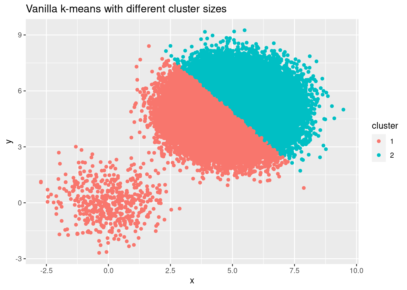
Consider the example from my last example, where we had two clusters, but with very different number of points in each of them (i.e. varying cluster cardinality). As the starting centers are chosen randomly, there is a high chance that both centers are chosen from the large cluster, which in turn leads to a completely wrong clustering in the end.
library(ggplot2)
library(gridExtra)

set.seed(2)
cluster_small <- data.frame(x = rnorm(500), y = rnorm(500))
cluster_large <- data.frame(x = rnorm(100000) + 5, y = rnorm(100000) + 5)
cluster_sizes <- rbind(cluster_small, cluster_large)
cluster_id_sizes <- kmeans(cluster_sizes, centers = 2)$cluster
## Warning: Quick-TRANSfer stage steps exceeded maximum (= 5025000)
ggplot(cluster_sizes, aes(x, y, color = factor(cluster_id_sizes))) +
  geom_point() +
  labs(title = "Vanilla k-means with different cluster sizes",
       color = "cluster")

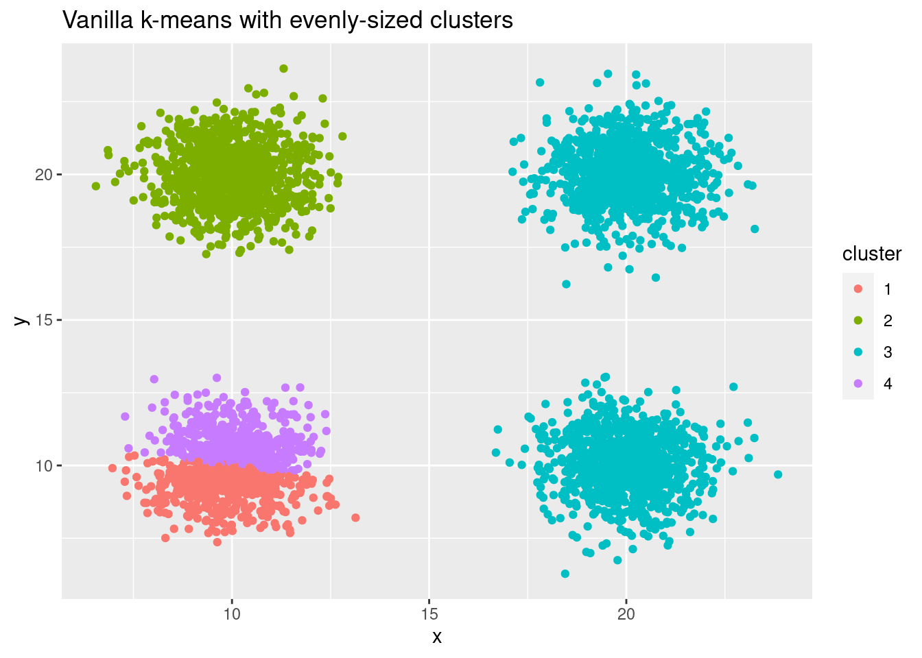
But also for evenly sized clusters we can get bad initialization, resulting in wrong outcomes:
cluster_multiple <- data.frame(x = rnorm(4000) + sample(seq(10, 20, 10), 4000, replace = TRUE),
                               y = rnorm(4000) + sample(seq(10, 20, 10), 4000, replace = TRUE))
cluster_id_multiple <- kmeans(cluster_multiple, centers = 4)$cluster
ggplot(cluster_multiple, aes(x, y, color = factor(cluster_id_multiple))) +
  geom_point() +
  labs(title = "Vanilla k-means with evenly-sized clusters",
       color = "cluster")

The k-means++ algorithm
A solution for this problem is the k-means++ algorithm, which uses a different initialization. The idea is pretty simple: Instead of random initialization, we only choose the first center randomly. All following centers are then still sampled, but with a probability that is proportional to their squared distance from all current centers. Points further away from current centers get a higher probability to become a center in the next iteration of initialization.
This attempts to fill the space of the observations more evenly, while still retaining some randomness. Even with k-means++, the outcome can differ between multiple runs on the same data. While it does require some more computation at the beginning of the algorithm, it leads to much faster convergence, making it highly competitive to vanilla k-means in regards to runtime. Therefore, many common libraries use k-means++ initialization as their default, for example sk-learn or the MatLab implementation.
Note that the distribution of the underlying data is only implicitly considered here, since the probability only relies on the distance to other centers, not on the distances to all other data points (in contrast to other initializations algorithms, such as partitioning around medoids). Still, areas with many points have a higher chance to create their own center, simply because more points could be chosen as a next center.
Implementation in R
The kmeans function shipped with base R actually has no k-means++
initialization option. So lets implement it, reusing the backbone of our
k-means algorithm from the last article. We will add an optional
argument to let the user choose the initialization, defaulting to the
k-means++ initialization we just discussed.
The first center is chosen randomly from the data. Then we create a centers data.frame, starting with the first center, and we will later fill with the remaining centers. At the same time we need to keep track of which points are not centers, to prevent us from choosing the same point again as a center.
next_center_id <- sample(seq_len(nrow(df)), 1)
centers <- df[next_center_id, ]
non_centers <- df[-next_center_id, ]
Next, we iteratively choose new centers according to their distance from
the current centers. We can use our helper function calculate_centers
from last time for this (if you dont know it anymore, see below in the
complete code), and we only need to consider the distance to the closest
center, so we call min on each row.
distances <- calculate_distances(non_centers, centers)
distances <- apply(distances, 1, min)
In the following step, we choose the next center according to the
distances. The sample function conveniently lets us specify the
probability for each point through the prob argument, and they don’t
even need to be between 0 and 1! So we could square our distances and
simply pass there, but to follow the original paper more closely, we do
the normalization as well:
probabilities <- distances^2 / sum(distances^2)
next_center_id <- sample(seq_len(nrow(non_centers)), 1, prob = probabilities)
Finally, we select the next center, append it to our centers data.frame and remove it from the non_centers data.frame.
next_center <- non_centers[next_center_id, ]
centers <- rbind(centers, next_center)
non_centers <- non_centers[-next_center_id, ]
We now only need to do this within a while loop, until we have chosen
as many centers as expected number of clusters k. This results in our
final function:
my_kmeans <- function(df, k, n_iterations, init = c("kmeans++", "random")) {
  # Check which initialization should be done
  init <- match.arg(init)

  # Helper function for euclidean distance
  euclidean_distance <- function(p1, p2) {
    dist <- sqrt(sum((p1-p2)^2))
    return(dist)
  }

  # Helper function to calculate distances between all points and all centers
  calculate_distances <- function(df, centers) {
    distances <- matrix(NA, nrow = nrow(df), ncol = nrow(centers))
    for (object_id in 1:nrow(df)) {
      for (center_id in 1:nrow(centers)) {
        distances[object_id, center_id] <- euclidean_distance(df[object_id, ], centers[center_id, ])
      }
    }
    return(distances)
  }

  if (init == "random") {
    # Choose all centers randomly
    centers <- df[sample(nrow(df), k, replace = FALSE), ]
  } else if (init == "kmeans++") {
    # Initialize according to kmeans++ algorithm

    # Choose first center randomly
    next_center_id <- sample(seq_len(nrow(df)), 1)
    centers <- df[next_center_id, ]
    non_centers <- df[-next_center_id, ]

    # Choose next centers with probabilities proportional to their distance to
    # the closest center. Higher distance equals higher probability.
    while(nrow(centers) < k) {
      distances <- calculate_distances(non_centers, centers)
      distances <- apply(distances, 1, min)
      # Choose point with maximum distance as next center
      next_center_id <- which.max(distances)
      # True k-means++ does the following:
      # probabilities <- distances/max(distances)
      # next_center_id <- sample(seq_len(nrow(non_centers)), 1, prob = probabilities)
      next_center <- non_centers[next_center_id, ]
      centers <- rbind(centers, next_center)
      non_centers <- non_centers[-next_center_id, ]
    }
  }

  # Perform n iterations
  iteration <- 1
  while(iteration < n_iterations) {
    # Calculate distance of each point to each center
    distances <- calculate_distances(df, centers)

    # Assign each point to the closest center
    cluster_id <- apply(distances, 1, which.min)

    # Calculate new centers
    for (i in seq_len(k)) {
      this_cluster <- df[cluster_id == i,]
      centers[k, ] <- colMeans(this_cluster)
    }

    iteration <- iteration + 1
  }

  return(cluster_id)
}
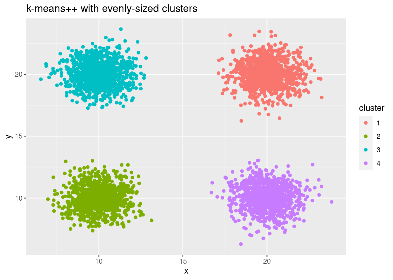
If we use the new kmeans++ initialization, we now recover correct clusters from the data:
cluster_id_multiple_kmeanspp <- my_kmeans(cluster_multiple, k = 4, n_iterations = 10, init = "kmeans++")
ggplot(cluster_multiple, aes(x, y, color = factor(cluster_id_multiple_kmeanspp))) +
  geom_point() +
  labs(title = "k-means++ with evenly-sized clusters",
       color = "cluster")

A common, but wrong k-means++ variant
As with many data science tools, there are also some variants floating around for the k-means++ technique. Quite frequently, it is described that it chooses the point with the largest distance to all other centers as the next center, instead of sampling with probabilities proportional to the distances. If you look at the original paper (link at the end of the article), this is not the true k-means++ algorithm and it also has a major disadvantage:
If one always chooses the center with the maximum distance, one can
easily select an outlier as the center. And as one typically chooses k
to be very small compared to the size of the data set, a handful of
outliers will be enough to only select outliers as initial centers! This
does not improve the clustering too much, as your main body of data has
no nicely distributed centers. Still, if you want to do it that way the
code within the while loop would look the following:
distances <- calculate_distances(non_centers, centers)
distances <- apply(distances, 1, min)
# Choose point with maximum distance as next center
next_center_id <- which.max(distances)
# True k-means++ does the following:
# probabilities <- distances/max(distances)
# next_center_id <- sample(seq_len(nrow(non_centers)), 1, prob = probabilities)
next_center <- non_centers[next_center_id, ]
centers <- rbind(centers, next_center)
non_centers <- non_centers[-next_center_id, ]
Summary
As we have seen, initialization can be key for the performance of k-means. The k-means++ algorithm is a simple and widely applied technique to alleviate the problems that vanilla k-means has. Some more other methods exist to further help with this, for example initializing the centers multiple times and selecting the initialization that has the lowest inertia. For example, sk-learn does 10 rounds of initialization by default.
For my use case, k-means++ unfortunately also was not enough and I needed even better methods. The most sophisticated initialization is probably contained in partitioning around medoids (PAM), which I will discuss in a following article. So stay tuned!
Sources
- Original paper describing the k-means++ algorithm: Arthur & Cassilvitskii (2007): k-means++: the advantages of careful seeding
- In case you dont have access to the paper, the math is also described in the MATLAB documentation
- Empirical evaluation of random initialization to k-means++
Photo by Braden Collum on Unsplash